Lab 2: Manipulator dynamics simulation

1. Install UMA manipulator package

You'll need to clone the uma_arm_description repository into your ROS2 workspace:

cd YOUR_ROS2_WS
cd src
git clone https://github.com/jmgandarias/uma_arm_description.git

Warning

This is a work-in-progress repository. Don't pay attention to the README.md file of that repo.

Info

You don't have to modify anything in this package. You just need it to visualize the manipulator.

Compile your workspace.

1.1. Test the UMA manipulator package

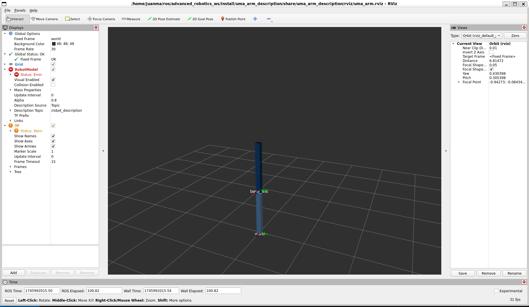
Open one terminal and run:

ros2 launch uma_arm_description uma_arm_visualization.launch.py

You'll see RViz2 opening and showing the following:

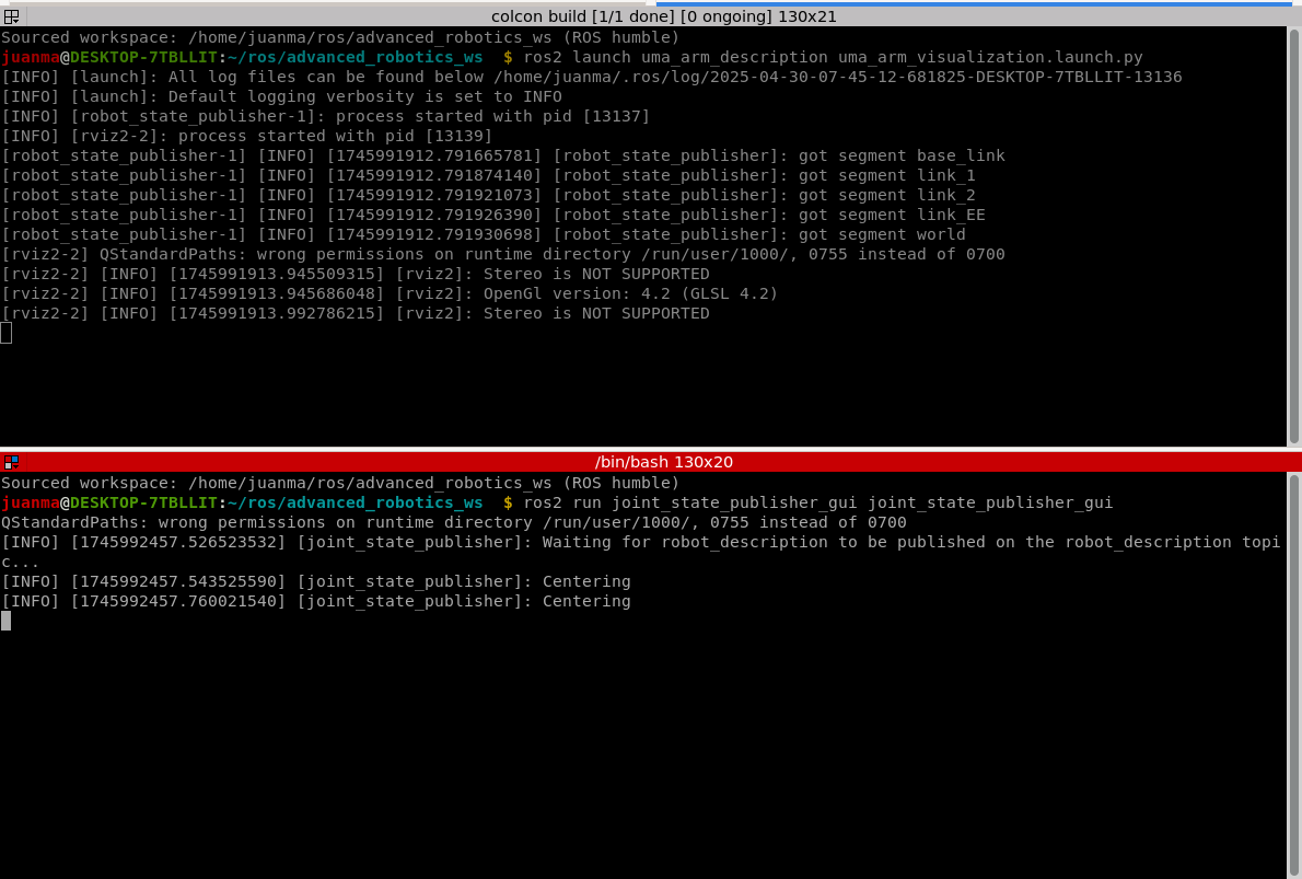
You can open a new terminal and run joint_state_publisher_gui to move the joints of the robot:

ros2 run joint_state_publisher_gui joint_state_publisher_gui 

Tip

If you press ctrl + shift + o or ctrl + shift + e in the terminator terminal, it will split the terminals vertically or horizontally

Now, you should have the following in your terminals

A GUI should have opened now allowing you to manually drive the joints of the manipulator

Success

Great work! Now you are ready to do the Lab session 2!

You can also close all the terminals (press ctrl + c).

---

2. Simulate the robot dynamics

The manipulator model you've loaded is purely a kinematic visualization (i.e., there is no dynamics - no forces, and there is no simulation)

Info

RViz 2 is a 3D visualization tool, not a simulator. It allows you to see robot models, sensor data, and other information shared in your ROS 2 environment in real time, and offers a GUI to select what to display, but it is NOT a simulator.

There are different ways to simulate the dynamics. The (probably) most straightforward one is to use a simulator such as Gazebo. However, as we are roboticists and want to see, touch, and learn the intrinsic effects of a manipulator's dynamics, we'll implement the dynamics (the equations of motion) of the manipulator as a ROS 2 node.

2.1. Clone the uma_arm_control package

To do this, we'll work with another package. You need to do the following:

cd YOUR_ROS2_WS
cd src
git clone https://github.com/jmgandarias/uma_arm_control.git

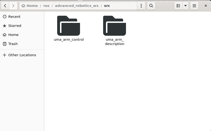
Once you have done this, your workspace folder should look like this

Tip

You can open the Ubuntu file manager even if you're using WSL, by running nautilus in a terminal:

nautilus

Now you can compile your workspace:

(If you're using the UMA environment, you can just do:)

cdw
cb

Success

Great work! You're now ready to implement the manipulator dynamics

But first, let's have a look at the uma_arm_control package distribution

2.2. Understanding the uma_arm_control package

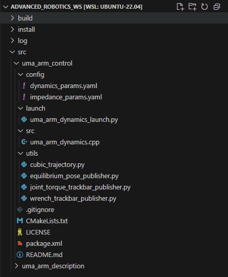
The package is structured as shown in the following image

Tip

You can directly open VSCode inside WSL by running code in a terminal

• config

  This folder contains configuration files that define various parameters.

  • dynamics_params.yaml: This file contains parameters related to the dynamics of the robotic arm. You need to modify it in this lab.
  • impedance_params.yaml: This file includes parameters for the impedance controller. You'll need to modify it in future sessions.

• launch

  This folder contains launch scripts.

  • uma_arm_dynamics_launch.py: This Python script launches the dynamics simulation node for the robotic arm. You don't have to modify it.

• src

  This folder contains the source code for the dynamics control and simulation of the robotic arm:

  • uma_arm_dynamics.cpp: This C++ file contains the implementation of the dynamics equations (equations of motion) for the robotic arm. You need to modify it in this lab.

• utils: This folder contains utility scripts that provide additional functionalities for the labs. You don't have to modify it.

• .gitignore: Specifies which files and directories should be ignored by Git version control. You don't have to modify it.
• CMakeLists.txt: Contains instructions for building the project using CMake, a build system generator. You'll need to modify it in future sessions.
• LICENSE: The license file that specifies the terms under which the project can be used and distributed. You don't have to modify it.
• package.xml: Defines the package metadata for ROS, including dependencies and other information. You don't have to modify it.
• README.md: Provides an overview of the project, instructions for setup, usage, and other relevant information. You should modify it and keep it updated as you work on the lab sessions.

2.3. Understanding the uma_arm_dynamics.cpp code

2.3.1. Libraries

Includes the needed libraries. You don't have to modify it.

Show the code

libraries.cpp

    #include <rclcpp/rclcpp.hpp>
    #include <sensor_msgs/msg/joint_state.hpp>
    #include <std_msgs/msg/float64_multi_array.hpp>
    #include <geometry_msgs/msg/wrench.hpp>
    #include <chrono>
    #include <Eigen/Dense>
    #include <cmath>

    using namespace std::chrono;

2.3.2. Constructor

ManipulatorDynamicsNode: Inherits from rclcpp::Node, making it a ROS 2 node. The class ManipulatorDynamicsNode is a ROS 2 node responsible for computing the dynamics of the manipulator (robot arm). You don't have to modify it.

ManipulatorDynamicsNode(): Class constructor that initializes the node with the name manipulator_dynamics_node.

Show the code

constructor_initialization

    class ManipulatorDynamicsNode : public rclcpp::Node
    {
    public:
        ManipulatorDynamicsNode()
            : Node("manipulator_dynamics_node"),
              joint_positions_(Eigen::VectorXd::Zero(2)),
              joint_velocities_(Eigen::VectorXd::Zero(2)),
              joint_accelerations_(Eigen::VectorXd::Zero(2)),
              joint_torques_(Eigen::VectorXd::Zero(2)),
              external_wrenches_(Eigen::VectorXd::Zero(2)),
              previous_time_(high_resolution_clock::now())
        {
            // Frequency initialization
            this->declare_parameter<double>("frequency", 1000.0);

            // Dynamics parameters initialization
            this->declare_parameter<double>("m1", 1.0);
            this->declare_parameter<double>("m2", 1.0);
            this->declare_parameter<double>("l1", 1.0);
            this->declare_parameter<double>("l2", 1.0);
            this->declare_parameter<double>("b1", 1.0);
            this->declare_parameter<double>("b2", 1.0);
            this->declare_parameter<double>("g", 9.81);
            this->declare_parameter<std::vector<double>>("q0", {0, 0});

            // Get frequency [Hz] parameter and compute period [s]
            double frequency = this->get_parameter("frequency").as_double();

            // Get dynamic parameters
            m1_ = this->get_parameter("m1").as_double();
            m2_ = this->get_parameter("m2").as_double();
            l1_ = this->get_parameter("l1").as_double();
            l2_ = this->get_parameter("l2").as_double();
            g_ = this->get_parameter("g").as_double();
            b1_ = this->get_parameter("b1").as_double();
            b2_ = this->get_parameter("b2").as_double();

            // Set initial joint position
            joint_positions_ = Eigen::VectorXd::Map(this->get_parameter("q0").as_double_array().data(), 2);

Member variables initialization

• joint_positions_, joint_velocities_, joint_accelerations_, joint_torques_, external_wrenches_: These are Eigen vectors initialized to zero. We'll use the library Eigen to work with vectors and matrices in C++.
• previous_time_: Initialized to the current time using high_resolution_clock::now().

Parameters declaration

• frequency: The frequency at which the node operates (default 1000 Hz).
• m1, m2: Masses of the manipulator's links.
• l1, l2: Lengths of the manipulator's links.
• b1, b2: Damping coefficients.
• g: Gravitational acceleration.
• q0: Initial joint positions.

Parameters Retrieval

• get_parameter: Retrieves the values of the declared parameters and assigns them to member variables. The values of the parameters are defined in the dynamics_params.yaml file inside the config folder.

Setting Initial Joint Positions

• joint_positions_: Sets the initial joint positions using the parameter q0.

Show the code

constructor_publisher_subscriber

     // Create subscription to joint_torques
     joint_torques_subscription_ = this->create_subscription<std_msgs::msg::Float64MultiArray>(
        "joint_torques", 1, std::bind(&ManipulatorDynamicsNode::joint_torques_callback, this, std::placeholders::_1));

    // Create subscription to external wrenches
    external_wrenches_subscription_ = this->create_subscription<geometry_msgs::msg::Wrench>(
        "external_wrenches", 1, std::bind(&ManipulatorDynamicsNode::external_wrenches_callback, this, std::placeholders::_1));

    // Create publisher for joint acceleration
    publisher_acceleration_ = this->create_publisher<std_msgs::msg::Float64MultiArray>("joint_accelerations", 1);

    // Create publisher for joint state
    publisher_joint_state_ = this->create_publisher<sensor_msgs::msg::JointState>("joint_states", 1);

    // Set the timer callback at a period (in milliseconds, multiply it by 1000)
    timer_ = this->create_wall_timer(
        std::chrono::milliseconds(static_cast<int>(1000 / frequency)), std::bind(&ManipulatorDynamicsNode::timer_callback, this));
    }

Subscriptions

• joint_torques_subscription_: Subscribes to the joint_torques topic, which is expected to publish messages of type std_msgs::msg::Float64MultiArray. The callback function joint_torques_callback is bound to handle incoming messages.
• external_wrenches_subscription_: Subscribes to the external_wrenches topic, which is expected to publish messages of type geometry_msgs::msg::Wrench. The callback function external_wrenches_callback is bound to handle incoming messages.

Publishers

• publisher_acceleration_: Creates a publisher for the joint_accelerations topic, which will publish messages of type std_msgs::msg::Float64MultiArray.
• publisher_joint_state_: Creates a publisher for the joint_states topic, which will publish messages of type sensor_msgs::msg::JointState.

Timer

• timer_: Sets up a timer that triggers the timer_callback function (explained below) at a period determined by the frequency parameter. The period is expected to be given in milliseconds, therefore, it is calculated as

\[ period \, \text{[ms]} = \frac{1 \, [\cancel{\text{s}}] \cdot 1000 \, [\text{ms}/\cancel{\text{s}}]}{frequency \, [\text{Hz}]} \]

2.3.3. Timer callback

The timer_callback function is responsible for:

• Calculating the elapsed_time_ between callbacks.
• Updating the new joint_accelerations_, joint_velocities_, and joint_positions_ using the respective functions (you'll need to implement these functions later).
• Publishing the updated joint states to the ROS topics.

This function ensures that the manipulator's state is updated and communicated at regular intervals based on the timer's frequency.

Show the code

timer_callback

    // Timer callback - when there is a timer callback, computes the new joint acceleration, velocity and position and publishes them
    void timer_callback()
    {
    // Get the actual elapsed time
    auto current_time = high_resolution_clock::now();
    elapsed_time_ = duration_cast<duration<double>>(current_time - previous_time_).count();
    previous_time_ = current_time;

    // Calculate JointState
    joint_accelerations_ = calculate_acceleration();
    joint_velocities_ = calculate_velocity();
    joint_positions_ = calculate_position();

    // Publish data
    publish_data();
    }

2.3.4. Topic callbacks

These callback functions ensure that the node's state is updated with the latest data from the subscribed topics. Specifically:

• joint_torques_callback: Updates the joint_torques_ based on incoming messages.
• external_wrenches_callback: Updates the external_wrenches_ based on incoming messages.

Show the code

topic_callbacks

    private:
        // Subscription callback - when a new message arrives, updates joint_torques_
        void joint_torques_callback(const std_msgs::msg::Float64MultiArray::SharedPtr msg)
        {
            joint_torques_ = Eigen::VectorXd::Map(msg->data.data(), msg->data.size());
        }

        // Subscription callback - when a new message arrives, updates external_wrenches_
        void external_wrenches_callback(const geometry_msgs::msg::Wrench::SharedPtr msg)
        {
            auto forces = msg->force;
            external_wrenches_(0) = forces.x;
            external_wrenches_(1) = forces.y;
        }

2.3.5. Calculate acceleration

This method computes the joint_accelerations_ of the manipulator by considering the equations of motion, including inertia, Coriolis and centrifugal forces, friction, gravitational forces, and external torques. You have to implement it as explained later.

At the moment, the method returns \(\mathbf{\ddot{q}} = [0, 0]\).

Show the code

calculate_acceleration

    // Method to calculate joint acceleration
    Eigen::VectorXd calculate_acceleration()
    {

        // Initialize M, C, Fb, g_vec, J, and tau_ext

        // Initialize q1, q2, q_dot1, and q_dot2

        // Placeholder calculations for M, C, Fb, g, and tau_ext
        // Calculate matrix M

        // Calculate vector C (C is 2x1 because it already includes q_dot)

        // Calculate Fb matrix

        // Calculate g_vect

        // Calculate J

        // Calculate tau_ext

        // Calculate joint accelerations using the dynamic model: q'' = M^(-1)[tau - C(q,q')q' - Fbq' - g(q) + tau_ext]
        Eigen::VectorXd q_ddot(2);
        q_ddot << 0, 0;

        // Return joint accelerations
        return q_ddot;
    }

2.3.6. Integrate position and velocity

This method computes the joint velocities and positions by integrating over the elapsed time. You have to implement it as explained later.

At the moment, the methods return \(\mathbf{\dot{q}} = \mathbf{q} = [0, 0]\).

Show the code

Integrate_vel_pos

     // Method to calculate joint velocity
     Eigen::VectorXd calculate_velocity()
     {
         // Placeholder for velocity calculation
         // Integrate velocity over the time step (elapsed_time_)
         Eigen::VectorXd q_dot(2);
         q_dot << 0, 0;

         return q_dot;
     }

     // Method to calculate joint position
     Eigen::VectorXd calculate_position()
     {
         // Placeholder for position calculation
         // Integrate position over the time step (elapsed_time_)
         Eigen::VectorXd q(2);
         q << 0, 0;

         return q;
     }

2.3.7. Publish the data

This method is responsible for publishing the computed joint_accelerations_ and joint_state (joint_positions_ and joint_velocities_) to their respective topics.

Show the code

publish_data

    // Method to publish the joint data
    void publish_data()
    {
        // publish joint acceleration
        auto acceleration_msg = std_msgs::msg::Float64MultiArray();
        acceleration_msg.data.assign(joint_accelerations_.data(), joint_accelerations_.data() + joint_accelerations_.size());
        publisher_acceleration_->publish(acceleration_msg);

        // publish joint state
        auto joint_state_msg = sensor_msgs::msg::JointState();
        joint_state_msg.header.stamp = this->get_clock()->now();
        joint_state_msg.name = {"joint_1", "joint_2"}; // Replace with actual joint names
        joint_state_msg.position = {joint_positions_(0), joint_positions_(1)};
        joint_state_msg.velocity = {joint_velocities_(0), joint_velocities_(1)};
        publisher_joint_state_->publish(joint_state_msg);
    }

2.3.8. Member variables

Defines the member variables for the ManipulatorDynamicsNode class. Here's a detailed breakdown of these variables: Member Variables

Show the code

member_variables

    // Member variables
        // Publishers and subscribers
        rclcpp::Subscription<std_msgs::msg::Float64MultiArray>::SharedPtr joint_torques_subscription_;
        rclcpp::Subscription<geometry_msgs::msg::Wrench>::SharedPtr external_wrenches_subscription_;
        rclcpp::Publisher<std_msgs::msg::Float64MultiArray>::SharedPtr publisher_acceleration_;
        rclcpp::Publisher<sensor_msgs::msg::JointState>::SharedPtr publisher_joint_state_;
        rclcpp::TimerBase::SharedPtr timer_;

        // Joint variables
        Eigen::VectorXd joint_positions_;
        Eigen::VectorXd joint_velocities_;
        Eigen::VectorXd joint_accelerations_;
        Eigen::VectorXd joint_torques_;
        Eigen::VectorXd external_wrenches_;

        // dynamic parameters variables
        double m1_;
        double m2_;
        double l1_;
        double l2_;
        double b1_;
        double b2_;
        double g_;

        // Variable to store the previous callback time and elapsed time
        time_point<high_resolution_clock> previous_time_;
        double elapsed_time_;
    };

Publishers and Subscribers

• joint_torques_subscription_: Subscription to the "joint_torques" topic.
• external_wrenches_subscription_: Subscription to the "external_wrenches" topic.
• publisher_acceleration_: Publisher for the "joint_accelerations" topic.
• publisher_joint_state_: Publisher for the "joint_states" topic.

Joint Variables

• joint_positions_: Eigen vector representing the positions of the joints (\(\mathbf{q}\)).
• joint_velocities_: Eigen vector representing the velocities of the joints (\(\mathbf{\dot{q}}\)).
• joint_accelerations_: Eigen vector representing the accelerations of the joints (\(\mathbf{\ddot{q}}\)).
• joint_torques_: Eigen vector representing the torques applied to the joints (\(\boldsymbol{\tau}\)).
• external_wrenches_: Eigen vector representing the external forces and torques applied to the EE (\(\mathbf{F}_{ext}\)).

Dynamic Parameters Variables

• m1_: Mass of the first link of the manipulator.
• m2_: Mass of the second link of the manipulator.
• l1_: Length of the first link of the manipulator.
• l2_: Length of the second link of the manipulator.
• b1_: Damping coefficient for the first joint.
• b2_: Damping coefficient for the second joint.
• g_: Gravitational acceleration.

Time Variables

• timer_: Timer that triggers the timer_callback function at a specified frequency.
• previous_time_: Stores the time of the previous callback execution.
• elapsed_time_: Stores the elapsed time between the current and previous callback executions (\(\Delta t\)).

2.3.9. Main

Initializes the ROS 2 node, creates a shared pointer to an instance of the ManipulatorDynamicsNode class, keeps the node running, and shuts down the ROS 2 node when the node execution finishes.

Show the code

main

    int main(int argc, char *argv[])
    {
        rclcpp::init(argc, argv);
        auto node = std::make_shared<ManipulatorDynamicsNode>();
        rclcpp::spin(node);
        rclcpp::shutdown();
        return 0;
    }

2.4. Implementing the dynamics model

The dynamics of an open kinematic chain robotic manipulator is given by

\[ \mathbf{M}(\mathbf{q}) \ddot{\mathbf{q}} + \mathbf{C}(\mathbf{q}, \dot{\mathbf{q}}) \dot{\mathbf{q}} + \mathbf{F}_b \dot{\mathbf{q}} + \mathbf{g}(\mathbf{q}) = \boldsymbol{\tau} + \boldsymbol{\tau}_{ext} \]

where

• \(\mathbf{q} \in \mathbb{R}^{n \times 1}\) is the vector of joint positions (joint_positions_).
• \(\dot{\mathbf{q}} \in \mathbb{R}^{n \times 1}\) is the vector of joint velocities (joint_velocities_).
• \(\ddot{\mathbf{q}} \in \mathbb{R}^{n \times 1}\) is the vector of joint accelerations (joint_accelerations_).
• \(\mathbf{M}(\mathbf{q}) \in \mathbb{R}^{n \times n}\) is the inertia matrix.
• \(\mathbf{C}(\mathbf{q}, \dot{\mathbf{q}}) \in \mathbb{R}^{n \times n}\) is the Coriolis and centrifugal forces matrix.
• \(\mathbf{F}_b \in \mathbb{R}^{n \times n}\) is the viscous friction matrix.
• \(\mathbf{g} \in \mathbb{R}^{n \times 1}\) is the gravity vector.
• \(\boldsymbol{\tau} \in \mathbb{R}^{n \times 1}\) is the vector of commanded joint torques (joint_torques_).
• \(\boldsymbol{\tau}_{ext} \in \mathbb{R}^{n \times 1}\) is the vector of joint torques due to external forces.

In our case, as we have a 2 DoF manipulator, \(n=2\).

Hence, the acceleration due to applied torques is given by

\[ \ddot{\mathbf{q}} = \mathbf{M}^{-1}(\mathbf{q}) \left[ \boldsymbol{\tau} + \boldsymbol{\tau}_{ext} - \mathbf{C}(\mathbf{q}, \dot{\mathbf{q}}) \dot{\mathbf{q}} - \mathbf{F}_b \dot{\mathbf{q}} - \mathbf{g}(\mathbf{q}) \right] \]

To calculate the joint accelerations, we first need to compute the matrices. They can be computed applying the Lagrange or the Newton-Euler formulations. In our case, the matrices are defined by:

\[ \mathbf{M}(\mathbf{q}) =\begin{bmatrix} & \\ m_1 \cdot l_1^2 + m_2 \cdot (l_1^2 + 2 \cdot l_1 \cdot l_2 \cdot \cos(q_2) + l_2^2) & m_2 \cdot (l_1 \cdot l_2 \cdot \cos(q_2) + l_2^2) \\ m_2 \cdot (l_1 \cdot l_2 \cdot \cos(q_2) + l_2^2) & m_2 \cdot l_2^2\\ & \\ \end{bmatrix} \]

\[ \mathbf{C}(\mathbf{q}, \dot{\mathbf{q}}) \dot{\mathbf{q}} = \begin{bmatrix} & \\ -m_2 \cdot l_1 \cdot l_2 \cdot \sin(q_2) \cdot (2 \cdot \dot{q}_1 \cdot \dot{q}_2 +\dot{q}_2^2) \\ m_2 \cdot l_1 \cdot l_2 \cdot \dot{q}_1^2 \cdot \sin(q_2)\\ & \\ \end{bmatrix} \]

\[ \mathbf{F}_b = \begin{bmatrix} & \\ b_1 & 0\\ 0 & b_2\\ & \\ \end{bmatrix} \]

\[ \mathbf{g}(\mathbf{q}) = \begin{bmatrix} & \\ (m_1 + m_2) \cdot l_1 \cdot g_ \cdot \cos(q_1) + m_2 \cdot g_ \cdot l_2 \cdot \cos(q_1 + q_2) \\ m_2 \cdot g \cdot l_2 \cdot \cos(q_1 + q_2)\\ & \\ \end{bmatrix} \]

We'll also need to compute the Jacobian to include the external wrenches applied at the EE in our model:

\[ \mathbf{J}(\mathbf{q}) = \begin{bmatrix} & \\ -l_1 \cdot \sin(q_1) - l_2 \cdot \sin(q_1 + q_2) & -l_2 \cdot \sin(q_1 + q_2) \\ l_1 \cdot \cos(q_1) + l_2 \cdot \cos(q_1 + q_2) & l_2 \cdot \cos(q_1 + q_2)\\ & \\ \end{bmatrix} \]

Then, we can calculate \(\boldsymbol{\tau}_{ext}\) as

\[ \boldsymbol{\tau}_{ext} = \mathbf{J}(\mathbf{q})^T \cdot \mathbf{F}_{ext} \]

We can now code them as

// Initialize M, C, Fb, g_vec, J, and tau_ext
Eigen::MatrixXd M(2, 2);
Eigen::VectorXd C(2);
Eigen::MatrixXd Fb(2, 2);
Eigen::VectorXd g_vec(2);
Eigen::MatrixXd J(2, 2);
Eigen::VectorXd tau_ext(2);

// Initialize q1, q2, q_dot1, and q_dot2
double q1 = joint_positions_(0);
double q2 = joint_positions_(1);
double q_dot1 = joint_velocities_(0);
double q_dot2 = joint_velocities_(1);

// Placeholder calculations for M, C, Fb, g, and tau_ext
// Calculate matrix M
M(0, 0) = m1_ * pow(l1_, 2) + m2_ * (pow(l1_, 2) + 2 * l1_ * l2_ * cos(q2) + pow(l2_, 2));
M(0, 1) = m2_ * (l1_ * l2_ * cos(q2) + pow(l2_, 2));
M(1, 0) = M(0, 1);
M(1, 1) = m2_ * pow(l2_, 2);

// Calculate vector C (C is 2x1 because it already includes q_dot)
C << -m2_ * l1_ * l2_ * sin(q2) * (2 * q_dot1 * q_dot2 + pow(q_dot2, 2)),
m2_ * l1_ * l2_ * pow(q_dot1, 2) * sin(q2);

// Calculate Fb matrix
Fb << b1_, 0.0,
0.0, b2_;

// Calculate g_vect
g_vec << (m1_ + m2_) * l1_ * g_ * cos(q1) + m2_ * g_ * l2_ * cos(q1 + q2),
    m2_ * g_ * l2_ * cos(q1 + q2);

// Calculate J
J << -l1_ * sin(q1) - l2_ * sin(q1 + q2), -l2_ * sin(q1 + q2),
    l1_ * cos(q1) + l2_ * cos(q1 + q2), l2_ * cos(q1 + q2);

// Calculate tau_ext
tau_ext << J.transpose() * external_wrenches_;

// Calculate joint acceleration using the dynamic model: M * q_ddot = torque - C * q_dot - Fb * joint_velocities_ - g + tau_ext
Eigen::VectorXd q_ddot(2);
q_ddot << M.inverse() * (joint_torques_ - C - Fb * joint_velocities_ - g_vec + tau_ext);

return q_ddot;

Tip

I suggest you use VSCode and install the C/C++ Themes extension. Once installed, you can auto format the code (usually by pressing ctrl + shift + i)

As we are implementing a discrete system:

\[ \ddot{\mathbf{q}}_{k+1} = \mathbf{M}^{-1}(\mathbf{q}_k) \left[ \boldsymbol{\tau}_k + \boldsymbol{\tau}_{{ext}_k} - \mathbf{C}(\mathbf{q}_k, \dot{\mathbf{q}}_k) \dot{\mathbf{q}}_k - \mathbf{F}_b \dot{\mathbf{q}}_k - \mathbf{g}(\mathbf{q}_k) \right] \]

we can get the joint velocities and position by discrete integration over time as

\[ \dot{\mathbf{q}} = \int \ddot{\mathbf{q}} \, dt \implies \dot{\mathbf{q}}_{k+1} = \dot{\mathbf{q}}_k + \ddot{\mathbf{q}}_{k+1} \cdot \Delta t \]

\[ \mathbf{q} = \int \dot{\mathbf{q}} \, dt \implies \mathbf{q}_{k+1} = \mathbf{q}_k + \dot{\mathbf{q}}_{k+1} \cdot \Delta t \]

We can now code them as

// Method to calculate joint velocity
Eigen::VectorXd calculate_velocity()
{
    // Placeholder for velocity calculation
    // Integrate velocity over the time step (elapsed_time_)
    Eigen::VectorXd q_dot = joint_velocities_ + joint_accelerations_ * elapsed_time_;

    return q_dot;
}

// Method to calculate joint position
Eigen::VectorXd calculate_position()
{
    // Placeholder for position calculation
    // Integrate position over the time step (elapsed_time_)
    Eigen::VectorXd q = joint_positions_ + joint_velocities_ * elapsed_time_;

    return q;
}

---

3. Launch the dynamics simulator node

Once you have coded the dynamics, open a terminal and compile it:

cdw
cb

Success

Great! You've coded the manipulator dynamics and are now ready to launch the node to see how they work.

First, you'll need to launch the UMA manipulator (step 2.1.).

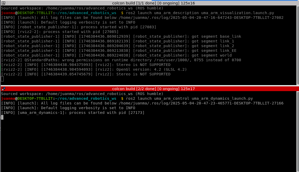
Hence, you will need to open 2 terminals and launch the following:

Terminal 1

Launch the UMA manipulator model uma_arm_visualization.launch.py:

ros2 launch uma_arm_description uma_arm_visualization.launch.py

Terminal 2

Launch the dynamics model uma_arm_dynamics_launch.py:

ros2 launch uma_arm_control uma_arm_dynamics_launch.py

Hence, you should see the following

And the result of the simulation is

Tip

• Note that the order in which you launch the scripts is important. You should first launch uma_arm_visualization. This loads the robot model, but it won't move until a message is published on the /joint_states topic.
• Then you can launch uma_arm_dynamics. This is what the dynamics model does: it computes the dynamic model and publishes the joint state to update the visualization. Note that the dynamics node doesn't require uma_arm_visualization to work. If you only launch the dynamics, they are computed without being shown in the visualizer. If you launch the visualization after starting the dynamics, the robot model will start updating immediately.

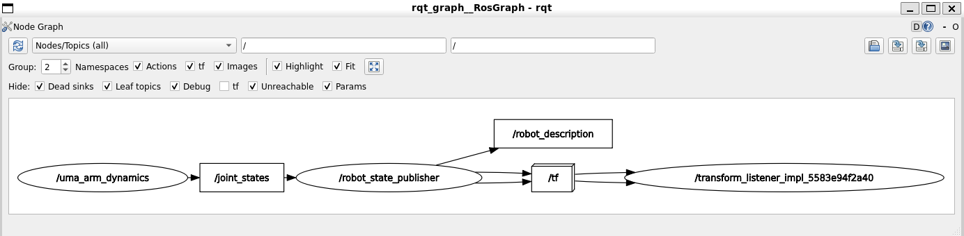
You can see the interaction between topics and nodes by opening another terminal and running:

rqt_graph

You have to select the option Node/Topics (all) and then update the graph.

---

4. Graphical representation

As robotics engineers, just seeing things work isn't enough for us. We want to understand how they work and be able to measure every parameter. One of the best ways to record the data of an experiment in ROS is to use ros bags.

To record the data of the experiment, you can do the following:

1. If you want to be organized, you can create an experiments folder to store the data there:

   cd
   mkdir experiments
   

2. Open a terminal and start the rosbag recording:

   cd
   cd experiments
   ros2 bag record --all -o experiment1
   ros2 bag record --all
   

3. Open another terminal and launch the UMA manipulator model:

   ros2 launch uma_arm_description uma_arm_visualization.launch.py
   

4. Open another terminal and launch the dynamics model uma_arm_dynamics_launch.py:

   ros2 launch uma_arm_control uma_arm_dynamics_launch.py
   

When the experiment is finished (for example, after around 15 seconds, when the manipulator is more or less steady), you can stop it by cancelling the recording and killing the nodes.

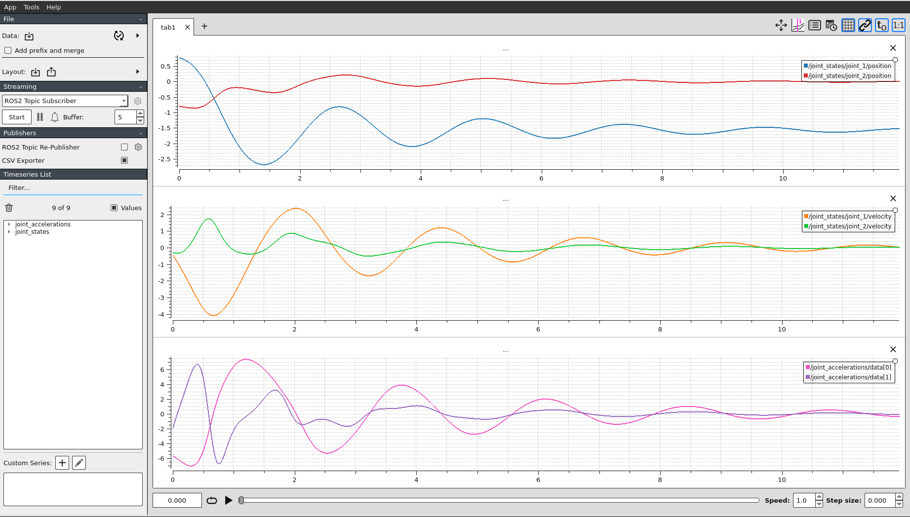
To represent time series of data in ROS 2, the uma_environment has installed the tool plotjuggler. You can find more information on how to use plotjuggler in this video.

You can run it using the corresponding UMA environment alias:

plotjuggler

Inside plotjuggler, and following the steps in the previous video, you can play the recorded rosbag. If you use the layout in pos_vel_acc_layout.xml, you can plot the joint positions, velocities, and accelerations.

Question

What are the effects of modifying the dynamics parameters of the arm?

You can modify some of the following parameters inside the dynamics_params.yaml: m1, m2, b1, b2, and g. Run different experiments and plot the data to see the effects of those parameters.

Note that you only need to modify those inside uma_arm_dynamics.

Nice plots and vector images

PlotJuggler is an excellent tool for visualizing ROS topic data, and it also offers options to manipulate data. However, sometimes you may want to use a more powerful tool such as MATLAB or Python (with matplotlib).

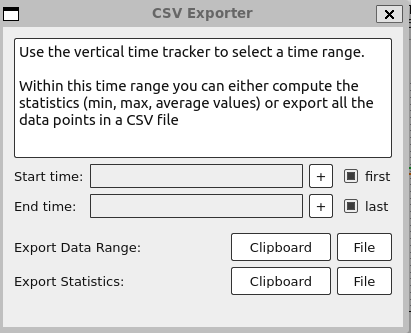
PlotJuggler allows you to save data in CSV format, which you can then easily import into your preferred software. Below is an example:

1. Click on the CSV exporter and export the data (export the data range into a file).

   

2. Go to MATLAB, open the CSV file, and select the data you want. In the figure below you can see how to select the timestamp (column A) and the joint position data for joint 1 (column F) and joint 2 (column H). Don't forget to exclude rows with non-importable cells. Then, select Import Selection as Generate Script to generate a script that imports your selected data.

   

   You'll probably need to modify that script to update the CSV file location or the name of the variable that stores your data. 4. Repeat these steps as many times as needed to get the data you want to plot. The MATLAB scripts to retrieve joint position, velocity, and acceleration data are provided below, respectively.

   • get_position_data.m
   • get_velocity_data.m
   • get_acceleration_data.m

3. Once you have the data in matlab, you can manipulate it the way you want. For example, you can create nicer plots with the units and names in the axes. Here I give you the script to create a nice plot with the experiment data.

   • plot_results.m

4. You can also export the figures in a vectorial graphic format such as PDF to have the best resolution possible, such as this one:

   

An alternative is to use the ROS Toolbox in MATLAB to read the recorded rosbag data directly. However, exporting via PlotJuggler is generally simpler.