Lab Session 5: Force Control

4.1. Introduction

In this lab, we will simulate the dynamic behavior of the RR manipulator under a force control scheme with an internal position loop. As in the previous lab sessions, the robot's dynamic behavior is linearized through the control law used in the previous labs:

\[ \boldsymbol{\tau} = \mathbf{M}(\mathbf{q}) \cdot \ddot{\mathbf{q}}_d + \underbrace{\mathbf{C} (\mathbf{q}, \dot{\mathbf{q}}) \cdot \dot{\mathbf{q}} + \mathbf{F}_b \cdot \dot{\mathbf{q}} + \mathbf{g}}_{\mathbf{n}(\mathbf{q}, \dot{\mathbf{q}})} + \mathbf{J}^T(\mathbf{q})\mathbf{f}_{e} \]

Note that the effect of external forces is also included in the compensation.

Hence, the manipulator follows a purely kinematic behavior expressed by the law:

\[ \ddot{\mathbf{q}} = \mathbf{J}(\mathbf{q})^{-1}[\ddot{\mathbf{x}} - \dot{\mathbf{J}}(\mathbf{q}, \dot{\mathbf{q}}) \dot{\mathbf{q}}] \]

In this case, the goal is to implement the force control law illustrated in the following diagram, according to the expression:

\[ \mathbf{M}_d\ddot{\mathbf{x}}_e + \mathbf{K}_D \dot{\mathbf{x}}_e + \mathbf{K}_P (\mathbf{I}_3 + \mathbf{C}_F \mathbf{K})\mathbf{x}_e = \mathbf{K}_P \mathbf{C}_F ( \mathbf{K} \mathbf{x}_r + \mathbf{f}_d) \]

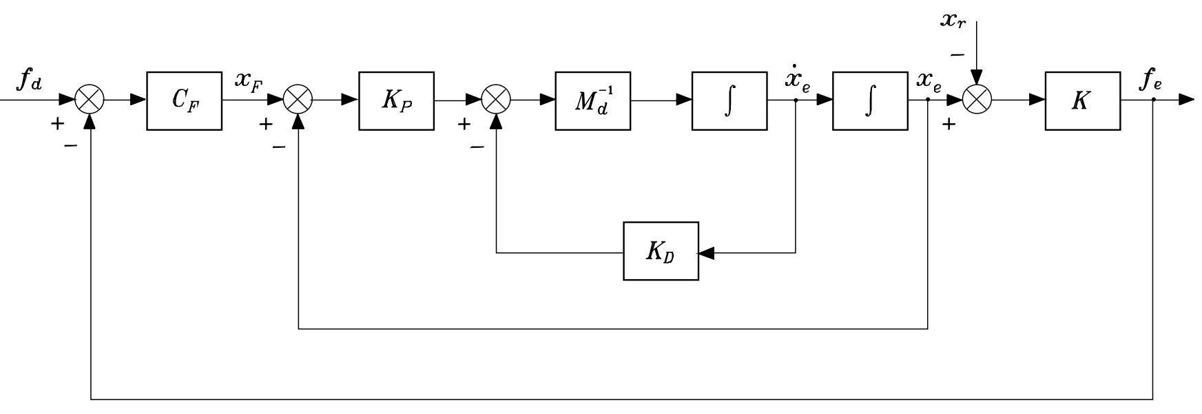
Here, the input signal to the system is now the reference force instead of a desired position. In the expression above, \(\mathbf{M}_d\), \(\mathbf{K}_P\), and \(\mathbf{K}_D\) retain the same meaning as the matrices \(\mathbf{M}\), \(\mathbf{B}\), and \(\mathbf{K}\), respectively.

The variable \(\mathbf{x}_F\) constitutes the system input and is defined as follows:

\[ \mathbf{x}_F = \mathbf{C}_F(\mathbf{f}_d - \mathbf{f}_e) \]

where $ \mathbf{C}_F$ is a proportional constant, \(\mathbf{f}_d\) is the reference force, and \(\mathbf{f}_e\) is the force applied by the robot on the elastic surface. In this way, if an elastic surface model is considered, it holds that:

\[ \mathbf{f}_e = \mathbf{K}(\mathbf{x}_e - \mathbf{x}_r) \]

Under these considerations, the following is requested:

4.2. Simulate P control

Simulate in SIMULINK the dynamic behavior of the manipulator in contact with the environment using the equivalent model, assuming the contact position is

\[ \mathbf{x}_r = [1.2,0.7] m \]

and the desired force is

\[ \mathbf{f}_d = [10, 0] N \]

when

\[ \mathbf{x}_{e_{initial}} = [1.3,0.7] m \, , \quad \mathbf{K} = \left[ \begin{matrix} & \\ 1000 & 0\\ 0 & 0\\ & \\ \end{matrix} \right] N/m \, , \quad \mathbf{C}_F = \left[ \begin{matrix} & \\ 0.05 & 0\\ 0 & 0\\ & \\ \end{matrix} \right] \]

and

\[ \mathbf{M}_d = \left[ \begin{matrix} & \\ 1000 & 0\\ 0 & 1000\\ & \\ \end{matrix} \right] N/m \, , \quad \mathbf{K}_D = \left[ \begin{matrix} & \\ 5000 & 0\\ 0 & 5000\\ & \\ \end{matrix} \right] N/m \, , \quad \mathbf{K}_P = \left[ \begin{matrix} & \\ 5000 & 0\\ 0 & 5000\\ & \\ \end{matrix} \right] N/m \]

Question

• Is the proposed controller correct? Why?
• What is happening in the Y axis? Why?

4.3. Simulate PI control

With the proposed control scheme, due to disturbances introduced by \(\mathbf{x}_r\), the reference force may not be reached in steady state. To address this, it is proposed to convert the constant \(\mathbf{C}_F\) into a proportional-integral action:

\[ \mathbf{C}_F = \mathbf{K}_F + \mathbf{K}_I \int^t (\cdot) d \varsigma \]

Implement this model in SIMULINK and simulate the dynamic behavior when

\[ \mathbf{K}_F = \left[ \begin{matrix} & \\ 0.03 & 0\\ 0 & 0\\ & \\ \end{matrix} \right] \, , \quad \mathbf{K}_I = \left[ \begin{matrix} & \\ 0.03 & 0\\ 0 & 0\\ & \\ \end{matrix} \right] \]

Question

• Does this produce any improvement in the controller? Why?
• Can you improve it more? How?